Example of model selection using cross-validation with RecTools

CV split
Training a variety of models
Measuring a variety of metrics

[1]:

from pprint import pprint

import numpy as np
import pandas as pd

from tqdm.auto import tqdm

from implicit.nearest_neighbours import TFIDFRecommender, BM25Recommender
from implicit.als import AlternatingLeastSquares

from rectools import Columns
from rectools.dataset import Dataset
from rectools.metrics import Precision, Recall, MeanInvUserFreq, Serendipity, calc_metrics
from rectools.models import ImplicitItemKNNWrapperModel, RandomModel, PopularModel
from rectools.model_selection import TimeRangeSplitter, cross_validate
from rectools.visuals import MetricsApp

Load data

[2]:

%%time
!wget -q https://files.grouplens.org/datasets/movielens/ml-1m.zip -O ml-1m.zip
!unzip -o ml-1m.zip
!rm ml-1m.zip

Archive:  ml-1m.zip
  inflating: ml-1m/movies.dat
  inflating: ml-1m/ratings.dat
  inflating: ml-1m/README
  inflating: ml-1m/users.dat
CPU times: user 144 ms, sys: 49.7 ms, total: 194 ms
Wall time: 4.35 s

[3]:

%%time
ratings = pd.read_csv(
    "ml-1m/ratings.dat",
    sep="::",
    engine="python",  # Because of 2-chars separators
    header=None,
    names=[Columns.User, Columns.Item, Columns.Weight, Columns.Datetime],
)
print(ratings.shape)
ratings.head()

(1000209, 4)
CPU times: user 7.42 s, sys: 222 ms, total: 7.64 s
Wall time: 7.67 s

[3]:

	user_id	item_id	weight	datetime
0	1	1193	5	978300760
1	1	661	3	978302109
2	1	914	3	978301968
3	1	3408	4	978300275
4	1	2355	5	978824291

[4]:

ratings["user_id"].nunique(), ratings["item_id"].nunique()

[4]:

(6040, 3706)

[5]:

ratings["weight"].value_counts()

[5]:

weight
4    348971
3    261197
5    226310
2    107557
1     56174
Name: count, dtype: int64

[6]:

ratings["datetime"] = pd.to_datetime(ratings["datetime"] * 10 ** 9)
print("Time period")
ratings["datetime"].min(), ratings["datetime"].max()

Time period

[6]:

(Timestamp('2000-04-25 23:05:32'), Timestamp('2003-02-28 17:49:50'))

Create Dataset class. It’s a wrapper for interactions. User and item features can also be added (see next examples for details).

[7]:

%%time
dataset = Dataset.construct(ratings)

CPU times: user 78.5 ms, sys: 3.88 ms, total: 82.4 ms
Wall time: 90.2 ms

Prepare cross-validation splitter

We’ll use last 3 periods of 2 weeks to validate our models.

[8]:

n_splits = 3

splitter = TimeRangeSplitter(
    test_size="14D",
    n_splits=n_splits,
    filter_already_seen=True,
    filter_cold_items=True,
    filter_cold_users=True,
)

[9]:

splitter.get_test_fold_borders(dataset.interactions)

[9]:

[(Timestamp('2003-01-18 00:00:00'), Timestamp('2003-02-01 00:00:00')),
 (Timestamp('2003-02-01 00:00:00'), Timestamp('2003-02-15 00:00:00')),
 (Timestamp('2003-02-15 00:00:00'), Timestamp('2003-03-01 00:00:00'))]

For test folds left border is always included in fold and the right one is excluded.

Train folds don’t have left border, and the right one is always excluded.

Train models

[10]:

# Take few simple models to compare
models = {
    "random": RandomModel(random_state=42),
    "popular": PopularModel(),
    "most_rated": PopularModel(popularity="sum_weight"),
    "tfidf_k=5": ImplicitItemKNNWrapperModel(model=TFIDFRecommender(K=5)),
    "tfidf_k=10": ImplicitItemKNNWrapperModel(model=TFIDFRecommender(K=10)),
    "bm25_k=10_k1=0.05_b=0.1": ImplicitItemKNNWrapperModel(model=BM25Recommender(K=5, K1=0.05, B=0.1)),
}

# We will calculate several classic (precision@k and recall@k) and "beyond accuracy" metrics
metrics = {
    "prec@1": Precision(k=1),
    "prec@10": Precision(k=10),
    "recall@10": Recall(k=10),
    "novelty@10": MeanInvUserFreq(k=10),
    "serendipity@10": Serendipity(k=10),
}

K_RECS = 10

[11]:

%%time

# For each fold generate train and test part of dataset
# Then fit every model, generate recommendations and calculate metrics

cv_results = cross_validate(
    dataset=dataset,
    splitter=splitter,
    models=models,
    metrics=metrics,
    k=K_RECS,
    filter_viewed=True,
)

CPU times: user 27 s, sys: 208 ms, total: 27.2 s
Wall time: 14.8 s

We can get some split stats

[12]:

pd.DataFrame(cv_results["splits"])

[12]:

	i_split	start	end	train	train_users	train_items	test	test_users	test_items
0	0	2003-01-18	2003-02-01	998083	6040	3706	630	75	540
1	1	2003-02-01	2003-02-15	998713	6040	3706	899	57	704
2	2	2003-02-15	2003-03-01	999612	6040	3706	597	66	501

And the main result is metrics

[13]:

pd.DataFrame(cv_results["metrics"])

[13]:

	model	i_split	prec@1	prec@10	recall@10	novelty@10	serendipity@10
0	random	0	0.000000	0.002667	0.000832	6.520987	0.000422
1	popular	0	0.053333	0.024000	0.037410	1.580736	0.000123
2	most_rated	0	0.053333	0.026667	0.042251	1.592543	0.000151
3	tfidf_k=5	0	0.053333	0.021333	0.023866	2.361189	0.000465
4	tfidf_k=10	0	0.026667	0.021333	0.039926	2.137451	0.000327
5	bm25_k=10_k1=0.05_b=0.1	0	0.026667	0.029333	0.046645	1.781881	0.000271
6	random	1	0.017544	0.005263	0.000732	6.490783	0.000605
7	popular	1	0.052632	0.057895	0.015707	1.588414	0.000183
8	most_rated	1	0.035088	0.056140	0.009919	1.600628	0.000155
9	tfidf_k=5	1	0.052632	0.057895	0.048591	2.326116	0.002616
10	tfidf_k=10	1	0.052632	0.052632	0.010033	2.143504	0.000917
11	bm25_k=10_k1=0.05_b=0.1	1	0.070175	0.059649	0.010321	1.809416	0.000341
12	random	2	0.015152	0.003030	0.000877	6.336690	0.000579
13	popular	2	0.045455	0.042424	0.039984	1.656638	0.000450
14	most_rated	2	0.045455	0.039394	0.024521	1.668108	0.000332
15	tfidf_k=5	2	0.090909	0.050000	0.039606	2.378988	0.001500
16	tfidf_k=10	2	0.060606	0.051515	0.053531	2.206921	0.001346
17	bm25_k=10_k1=0.05_b=0.1	2	0.090909	0.039394	0.038426	1.901316	0.000397

Let’s now aggregate metrics by folds and compare models

[14]:

pivot_results = (
    pd.DataFrame(cv_results["metrics"])
    .drop(columns="i_split")
    .groupby(["model"], sort=False)
    .agg(["mean"])
)
pivot_results.columns = pivot_results.columns.droplevel(1)

(
    pivot_results.style
    .set_caption("Mean values of metrics")
    .highlight_min(color='lightcoral', axis=0)
    .highlight_max(color='lightgreen', axis=0)
)

[14]:

Mean values of metrics
	prec@1	prec@10	recall@10	novelty@10	serendipity@10
model
random	0.010898	0.003653	0.000813	6.449487	0.000535
popular	0.050473	0.041440	0.031034	1.608596	0.000252
most_rated	0.044625	0.040734	0.025564	1.620426	0.000213
tfidf_k=5	0.065625	0.043076	0.037354	2.355431	0.001527
tfidf_k=10	0.046635	0.041827	0.034497	2.162626	0.000863
bm25_k=10_k1=0.05_b=0.1	0.062584	0.042792	0.031797	1.830871	0.000337

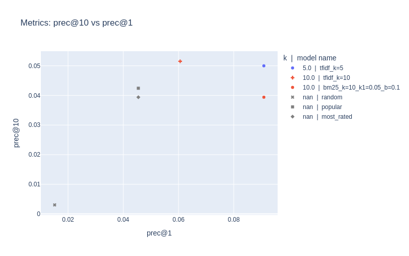
In RecTools we have interactive MetricsApp for detailed analysis of metrics trade-off between different models. visuals extension is required to run the path of code below. You can install it with pip install rectools[visuals]

[15]:

metadata_example = {
    Columns.Model: ["random", "popular", "most_rated", "tfidf_k=5", "tfidf_k=10", "bm25_k=10_k1=0.05_b=0.1"],
    "k": [None, None, None, 5, 10, 10]
}

[16]:

app = MetricsApp.construct(
    models_metrics=pd.DataFrame(cv_results["metrics"]),
    models_metadata=pd.DataFrame(metadata_example),  # optional
)

If you run this notebook, you will get interactive widgets with active buttons to select metrics, folds and metadata coloring. For offline presentation we keep static screenshots of the actual app.

If you want to save static image from your app, you can access plotly.graph_objs.Figure and render it as an image. Make sure you have kaleido package to process rendering. You can install it with pip install kaleido==0.2.1 and restart the kernel.

[17]:

fig = app.fig
fig.update_layout(title="Metrics: prec@10 vs prec@1")
fig.show("png")

../_images/examples_2_cross_validation_31_0.png